Image Colorization Using Convolutional Neural Network
This article introduces image Colorization based on Convolutional Neural Network
About Convolutional Neural Network
A convolutional neural network (CNN) is a type of deep learning model that can process images, speech, or other types of data that have a grid-like structure. CNNs are composed of layers that perform different operations on the input data, such as convolution, pooling, and fully-connected layers. CNNs can learn to extract features and patterns from the data, and use them for tasks like image classification, object detection, face recognition, and more.
About CNN-based Image Colorization
Image colorization is the process of adding color to black and white images, usually old photographs or historical images. It can be done manually by artists, or automatically by using artificial intelligence algorithms. When dealing with image-processing tasks, CNN has the advantages including less computation, less resource using, easier to train, and can be faster than other algorithms such as full-connected neural networks. However, although CNN is proved to be pretty suitable for tasks like image recognization, image feature extraction and image classification, it may not work as efficient as more advanced algorithms such as generative neural networks when doing more creative tasks like image colorization. However, we will still use CNN to achieve image colorization due to its simplicity.
Import libraries
import cv2
import numpy as np
import os
import matplotlib.pyplot as plt
import skimage
import skimage.color
import skimage.util
from collections import OrderedDict
import torch
import torch.nn as nn
import torch.nn.functional as f
import torch.utils.data as data
import pytorch_ssim
Set up parameters in training
batch_size = 4
epochs = 300
learning_rate = 0.0001
image_num = 4     # Number of images in training set
device = torch.device('cuda' if torch.cuda.is_available() else 'cpu')
Data preprocessing
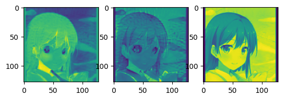
First thing we need to do is transform the image from RGB color domain to LAB color domain. This is because the channel L refers to the grey scale channel( or can be extracted from input easily ). By using this strategy, we only need to train channel a and channel b, which reduces resource consumption.
img_width = 128
img_height = 128
def rgb2lab(path, mode=0):
    img = skimage.io.imread(path)
    img = cv2.resize(img, (img_width, img_height), interpolation=cv2.INTER_AREA)
    img_lab = skimage.color.rgb2lab(img)
    L, a, b = cv2.split(img_lab)
    L = skimage.util.img_as_float(L)/100
    a = skimage.util.img_as_float(a)/128
    b = skimage.util.img_as_float(b)/128
    if(mode == 0):
        return L
    elif(mode == 1):
        img_ab = cv2.merge([a, b])
        return img_ab
    else:
        return img_lab

def lab2rgb(L, a, b):
    L = skimage.util.img_as_float(L) * 100
    a = skimage.util.img_as_float(a) * 128
    b = skimage.util.img_as_float(b) * 128
    img_lab = np.dstack((L, a, b))
    img_rgb = skimage.color.lab2rgb(img_lab)
    return img_rgb

i= 0
path_images = '../image/archive/out2/'
path_edges = '../image_edges/'
imageset = []
edgeset = []
image_labels = os.listdir(path_images)
edge_labels = os.listdir(path_images)
# edge_labels = os.listdir(path_edges)

# Dimensions of training set:torch.Size([image_num+1, 256, 256, 3]); torch.Size([image_num+1, 256, 256])
for label1, label2 in zip(image_labels, edge_labels):
    imageset.append(rgb2lab(path_images + label2, mode = 1))   # Read in images as (a,b) channels and resize to (128, 128)
    edgeset.append(rgb2lab(path_images + label2, mode = 0))    # Read in images as (L) channel and resize to (128, 128)
    i += 1
    if(i >= image_num):
        break
plt.figure()
plt.subplot(1,3,1)
plt.imshow(imageset[0][:,:, 0])
plt.subplot(1,3,2)
plt.imshow(imageset[0][:,:, 1])
plt.subplot(1,3,3)
plt.imshow(edgeset[0])

imageset = torch.tensor(imageset)
edgeset = torch.tensor(edgeset)

loader = data.DataLoader(data.TensorDataset(imageset, edgeset), shuffle=True, batch_size=batch_size)
We can check whether our training data is well-done by looking through plotted figures:
Model construction
Our model consists of 9 layers, the first five layers are used to extracted features in images, and the last four layers are designed for down-sampling. Leaky-Relu actvation is used for conv2D in order to avoid gradient vanishing problem. Tahn activation is used in the last layer to nominize pixels to [-1, 1].
def make_layers(block):
    layers = []
    for layer_name, v in block.items():
        if 'pool' in layer_name:
            layer = nn.MaxPool2d(kernel_size=v[0], stride=v[1],
                                    padding=v[2])
            layers.append((layer_name, layer))
        else:
            conv2d = nn.Conv2d(in_channels=v[0], out_channels=v[1],
                               kernel_size=v[2], stride=v[3],
                               padding=v[4])
            layers.append((layer_name, conv2d))
            activation = nn.LeakyReLU()
            layers.append(('leakyrelu_'+ layer_name, activation))

    return nn.Sequential(OrderedDict(layers))

class Mymodel(nn.Module):
    def __init__(self):
        super(Mymodel, self).__init__()
        conv = OrderedDict([
            ('conv1', [1, 64, 3, 1, 1]),
            ('conv2', [64, 128, 3, 1, 1]),
#            ('pool1', [2, 2, 0]),
            ('conv3', [128, 256, 3, 1, 1]),
            ('conv4', [256, 512, 3, 1, 1]),
            ('conv5', [512, 512, 3, 1, 1]),
            ('conv6', [512, 256, 3, 1, 1]),
#            ('pool2', [2, 2, 0]),
            ('conv7', [256, 128, 3, 1, 1]),
            ('conv8', [128, 64, 3, 1, 1]),
        ])
        self.model_conv = make_layers(conv).to(device)
#        self.interpolate = nn.Upsample(scale_factor=8, mode="bilinear", align_corners=True).to(device)

        self.conv_out = nn.Sequential(
            nn.Conv2d(in_channels=64, out_channels=2, kernel_size=(3, 3), stride=(1, 1), padding=(1, 1)),
            nn.Tanh()
        )

    def forward(self, x):
        x1 = self.model_conv(x)
        conv_out = self.conv_out(x1)
        return conv_out


    def forward(self, x):
        x1 = self.model_conv(x)
        conv_out = self.conv_out(x1)
        return conv_out

model = Mymodel().to(device)
Training
Before training, we define a class for combination of loss functions:
class CombinedLoss(nn.Module):
    def __init__(self, alpha, beta, gamma):
        super(CombinedLoss, self).__init__()
        self.alpha = alpha
        self.beta = beta
        self.gamma = gamma
        self.l1_loss = nn.L1Loss()              # L-1 loss function
        self.l2_loss = nn.MSELoss()             # L-2 loss function
        self.ssim_loss = pytorch_ssim.SSIM()    # ssim loss function

    def forward(self, pred, target):
        l1 = self.l1_loss(pred, target)
        l2 = self.l2_loss(pred, target)
        ssim = 1 - self.ssim_loss(pred, target)
        loss = self.alpha * l1 + self.beta * l2 + self.gamma * ssim
        return loss
By adjusting values of alpha, beta and gamma, we can set up the best combined loss function. As an example, we use L-2 loss function while training.
# cost_function = CombinedLoss(alpha=0, beta=0.5, gamma=0.5)
cost_function = nn.MSELoss()
loss = 0
loss_print = []
optimizer = torch.optim.Adam(model.parameters(), lr=learning_rate)
We can also define a function for initializing parameters in our model. We do not use it at this time. The reason I put it here is for illumination.
# Function for initialization
def init_normal(m):
    if isinstance(m, nn.Conv2d):
        torch.nn.init.constant_ (m.weight, 0)
        torch.nn.init.constant_ (m.bias, 0)

# Applying initialization for all parameters in our model
model.apply(init_normal)
Now we can focusing on training our model:
# Training
for epoch in range(1, epochs+1):
print("================ EPOCH: " + str(epoch) + "================")
for data_batch in loader:
y_pred = model.forward((data_batch[1].unsqueeze(1).float().to(device)))
loss = cost_function(y_pred, (data_batch[0]).permute(0, 3, 1, 2).float().to(device))
print('Loss: ' + str(loss))
model.zero_grad()
loss.backward()
optimizer.step()
loss_print.append(loss)
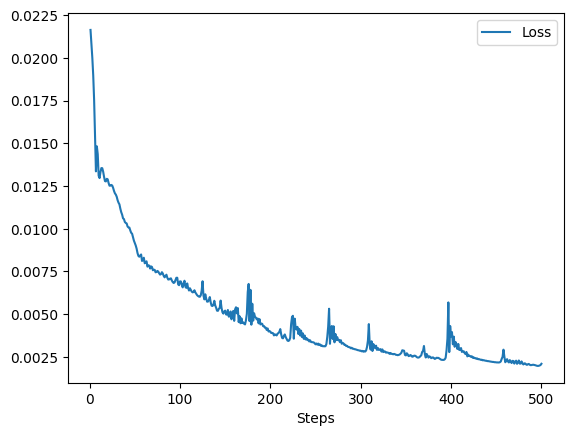
x = np.arange(1, len(loss_print) + 1, 1)
loss_print = [t.cpu().detach().numpy() for t in loss_print]
plt.figure()
plt.plot(x, loss_print[0:len(loss_print):1])
plt.legend(labels=["Loss"])
plt.xlabel("Steps")
plt.savefig('./Loss.jpg')
plt.show()
We need to censor the cost function with respect to training steps( or epochs )to make sure that our model is well-trained:
If everything goes well, stop training and save our model:
torch.save(model, 'model.pt')
Testing
In order to test our model, we will first reload our model:
model = torch.load('model.pt')
model.eval()
Then, read in images for testing and push these images into reloaded model. After getting results, we save them in a specific file folder.
for label1, label2 in zip(image_labels, edge_labels):
    image_test = rgb2lab(path_images + label2, mode=0)

    pred = model.forward(torch.tensor(image_test).unsqueeze(0).unsqueeze(0).float().to(device))
    pred = pred.cpu().detach().numpy()
    pred = lab2rgb(image_test, pred[0,0,:,:], pred[0,1,:,:])
    plt.imsave('../image_out/' + str(label2), pred)
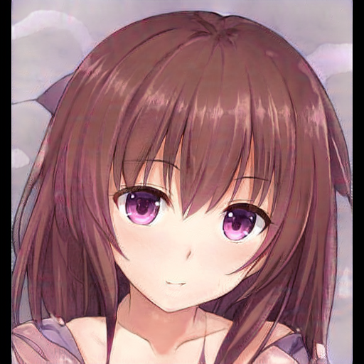
Now we can go to the folder and check the generated and saved images. I trained the model with about 300 epochs using only several images in an open-source dataset of anime character avatars. However, I will show that the model can actually work well even only several images are trained.
Original figures ( RGB figures, 512*512 ):


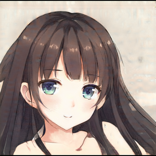
Generated figures ( RGB figures, 128*128 ):


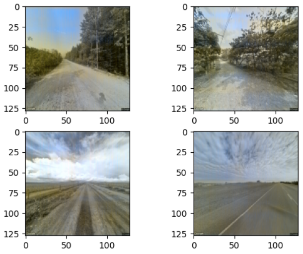
This model can also be used for other dataset. However, due to the limitations of network structure and training resources, it may not work well without optimizations. Here is can example, we use the model to colorize images of landscape:
Summary
From the results, we can see that our model is able to colorize anime character avatars, figures of landscope, etc. However, I found that convolutional neural networks are not so proficient with image colorization, especially when we are using a large amount of images for training, convolutional neural networks tend to ignore or overlook features in each images. In other words, the predictions are prone to be the same. This may because the model structure is not sensible, the hyper-parameters are not set adequately or the training set contains too much information that exceed the processing ability of this kind of structure. Although it has some drawbacks, due to its maturity, resources requirement and high speed on both training and utilization, CNN is still one of the most widely-used deep-learning algorithms for image processing.