Machine learning Algorithm - Linear Regression

What is linear regression

Linear regression is a statistical method used to model the relationship between a dependent variable and one or more independent variables. Linear regression aims at solving problems like predicting continuous valued label, that is, suppose we have a training dataset and each is represented as (x, y), x is the feature and y is the continuous valued label. After applying learning algorithm, our model will learn the function h(x): x -> y so that when new data appears, the model will predict the output value y by the input feature x.

Linear regression belongs to supervised learning, also known as supervised machine learning, which is a subcategory of machine learning and artificial intelligence. It is defined by its use of labeled datasets to train algorithms that to classify data or predict outcomes accurately.

Linear regression with one variable

The simplest example is linear regression with only one variable. Linear regression with one variable, also known as simple linear regression or univariate linear regression, is used to estimate the relationship between two quantitative variables. In this method, you have one independent variable (input) and one dependent variable (output). The independent variable is used to predict the value of the dependent variable.

Since there is only one input feature, We can define the hypothesis function h(x) as follows. In this function, m is the amount of data:

Now let’s consider how to choose parameters θj. Based on training set, we want to train the model to generate parameters θj so h(x) is close to the value y corresponding to input feature x.

Let’s use the function below as our cost funtion, which is also known as square error function:

This function measures the accuracy of our hypothesis. You can also choose other cost function according to the task. But remember that the cost function used for linear regression should always be a convex function.

In order to refresh parameters θj, we use gradient descent algorithm to minimize the cost function J(θ). We Start with initial guesses ( or randam numbers ) and keep changing θj a little bit to try and reduce J(θ). Since there is only one vairable, this process can be explained as below:

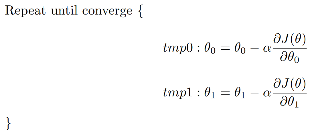
The derivation process in the formula is as follows:

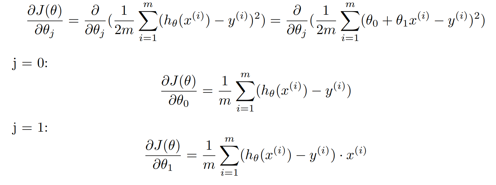
In the algorithm, α is the learning rate, which is a parameter we set to adjust the speed of gradient descent. If α is too small, the gradient descent will be too slow. If it is too large, gradient descent may overshoot minimum and not converge. α can be constant, but in practice, gradually decreasing α when approaching local minimum is more commonly-used.

Now what you need to do is just repeat until you converge to a local minimum.

linear regression with multiple variables

What if there are more variables or features? We can replace univariate functions with multivariate functions as our hypothesis function:

We ca also define our cost function as:

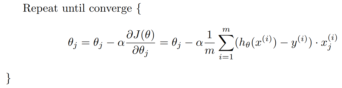
In order to refresh parameters θj, we use gradient descent algorithm again to minimize the cost function J(θ). You have to simultaneously update for every j = 0, 1, 2 …, n in a repeat.

Ways to improve gradient descent

1. Adjust learning rate α dynamically.
2. Use feature scaling, such as mean normalization.
3. Try polynomial regression, that is, using polynomial as hypothesis function h(x).
4. Use normal equation method. This method is quite useful when the dataset is small. However, with a large dataset, it may not be able to give us the best parameter of the model.