Programming Exercise for Linear Regression
This article is for Linear Regression Programming Exercise.
About linear regression
For the concept, mathematical derivation and optimization methods of linear regression, please view the previously posted article Machine learning Algorithm - Linear Regression.
Programming Exercise
Import libraries
import matplotlib.pyplot as plt
import numpy as np
Set up parameters in training
m = 500                      # Size of training set.
epochs = 5                   # Number of training epoch.
batch_sizes = 20             # Number of training elements in one batch.
iterations = int(m/batch_sizes)
lr = 0.001                   # Learning rage.
assert m % batch_sizes == 0  #Raising an AssertionError when m is not divisible by batch_sizes.
Generate training set
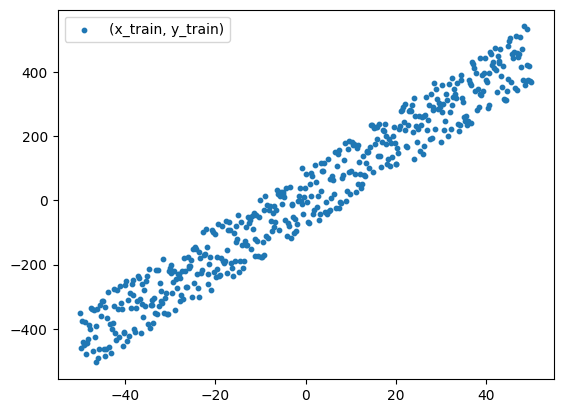
We generate m points near the objective function as our training set:
# Generate m pairs (x, y) as training set.
x1, x2, x3 = np.linspace(-50, 50, m).reshape((batch_sizes, iterations)), np.linspace(-50, 50, m).reshape((batch_sizes, iterations)), np.linspace(-50, 50, m).reshape((batch_sizes, iterations))
# Fitted objective function: y = 10 + 5 * x1 - 6 * x2 + 10 * x3
y = 10 + 5 * x1 - 6*x2 + 10 * x3 + np.random.rand(batch_sizes, iterations) * 200 - 100 # Introduce noise
x = np.linspace(-50, 50, m)
plt.scatter(x, y, s=10) # Visualize training set
plt.legend(["(x_train, y_train)"])
Now we can view the generated training set:
Training
# Initialize parameters
a0, a1, a2, a3 = np.random.rand(4)
d0, d1, d2, d3 = [0,0,0,0]
H = a0 + a1 * x1 + a2 * x2 + a3 * x3
J = 0 # Cost function
J_out = np.array([]) # Array used for plotting
# Training process
for epoch in range(0, epochs):
print("=============== Training epoch " + str(epoch) + "===============")
for batch_size in range(0, batch_sizes):
J = 0
d0, d1, d2, d3 = [0, 0, 0, 0]
H = a0 + a1 * x1 + a2 * x2 + a3 * x3
for iteration in range(0, iterations):
# Cost function and gradient descent
J = J + (1/(2 * m)) * ((H[batch_size][iteration] - y[batch_size][iteration]) ** 2)
d0 = d0 + (1 / m) * (H[batch_size][iteration] - y[batch_size][iteration])
d1 = d1 + (1 / m) * ((H[batch_size][iteration] - y[batch_size][iteration]) * x1[batch_size][iteration])
d2 = d2 + (1 / m) * ((H[batch_size][iteration] - y[batch_size][iteration]) * x2[batch_size][iteration])
d3 = d3 + (1 / m) * ((H[batch_size][iteration] - y[batch_size][iteration]) * x3[batch_size][iteration])
# Update parameters
a0 = a0 - lr * d0
a1 = a1 - lr * d1
a2 = a2 - lr * d2
a3 = a3 - lr * d3
# Update for plotting
J_out = np.append(J_out, J)
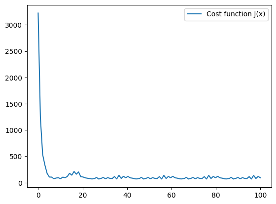
# Visualize cost function
plt.figure
plt.plot(np.linspace(0, epochs*batch_sizes, epochs*batch_sizes), J_out)
plt.legend(["Cost function J(x)"])
plt.show
Now we can view the cost function as we training the model to evaluate results of training:
Generate testing set and evaluate training results
Similarly, we generate our testing set:
# Generate testing set
x1_t, x2_t, x3_t = np.linspace(-50.5, 50.5, m), np.linspace(-50.5, 50.5, m), np.linspace(-50.5, 50.5, m)
y_hat = a0 + a1 * x1_t + a2 * x2_t + a3 * x3_t
x_t = np.linspace(-50.5, 50.5, m)
Then we can draw the hypothesis of our testing set and our training set in one figure to evaluate how our trained model works:
# Visualize testing set
plt.figure
plt.scatter(x, y, s=10)
plt.plot(x_t, y_hat, c="r")
plt.legend(["(x_train, y_train)","y_test"])
plt.show
Now we can view the results of our generated model (the red line):
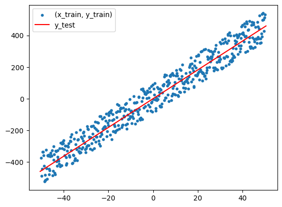
From the results, we can see that our model is able to successfully fit linear functions, which proves that linear regression model is great for fitting linear functions.