Machine learning Algorithm - Principal Component Analysis

Motivation of dimensionality reduction

We may want to reduce the dimension of features if we have too much redundant data. To do this, we can find two highly corelated features, plot them and make a new feature that can describe both features accurately. By doing this, we can reduce the total data we stored in memory and accelerate computing.

Another good example of dimensionality reduction is that it is not easy to visualize data that has more than three dimensions. We need to find new features (equal or less than three) to summarize all these features in the data set.

PCA Problem Formulation

Principal Component Analysis (PCA) is a statistical technique used to reduce the dimensionality of a dataset by transforming the data into a new coordinate system where the variation in the data can be described with fewer dimensions than the initial data. It is commonly used for dimensionality reduction by projecting each data point onto only the first few principal components to obtain lower-dimensional data while preserving as much of the data’s variation as possible.

The goal of PCA is to reduce the average of all the distances of all the features to the projection line, plane or higher dimensions. For instance, if we want to reduce our dimensions from 2d to 1d, then our goal is finding a new line and map our old features onto this new line to get a new feature while trying to reduce the average of all the distances of all the features to the new line.

Mathematical derivation of PCA algorithm

Matrix representation of vector basis transformation

From linear algebra we know that the inner product operation maps two vectors to a real number. Suppose we have vectors A and B, where B is a unit vector, then the inner product value of A and B is equal to the scalar size of the projection of A to B. We can draw the conclusion that to accurately describe a vector, we must first determine a set of basis vectors, and then determine the projection value of the vector in the direction of the basis vectors. The basis vectors are not required to be orthogonal, nor are the scalars required to be 1. But for convenience, we take the orthogonal unit vector as our basis vector.

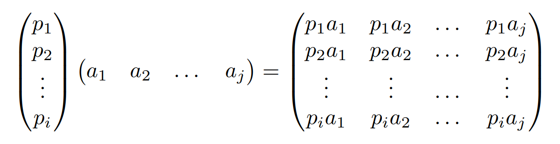
We can write the basis transformation of vectors in a general form, where pi is a row vector representing the i-th basis vector, and aj is a column vector representing the j-th original data:

Variance and covariance

If the dimensionality of basis vectors is lower than original vectors, then we can achieve dimensionality reduction. Now the question is how to choose basis vectors to retain the original information to the maximum extent. We can use variance to evaluate the quality of selected basis vectors. This is because the degree of dispersion of values can be expressed as mathematical variance, and we want the projected vector to be as dispersed as possible, that is, to have greater entropy. According to Shannon information theory, greater entropy means that the data can carry much information, in other words, less information loss.

What’s more, in order to represent as much original information as possible, we hope that there will be no linear correlation between these variables, because correlation means that these variables are not linearly independent, and there must be repeated representation of information. We can use covariance to evaluate correlation between variables. In this example, we hope that the covariances of these variables are equal to 0.

Now the solution is much clear: To reduce a set of N-dimensional vectors to K-dimensional, our goal is to select K unit orthogonal vector bases so that after the original data is transformed to this set of vector bases, the covariance between each variable is 0, and the variance of the variables is as large as possible.

Covariance matrix and matrix diagonalization

Let’s first have a close look at covariance of two variables. The covariance of two variables is defined as follows. Since m is the number of sample bodies, which is a very large number, and we preprocess the data so that the mean of the data is 0, the covariance of variable a and b can be simplified.

Similarly, if we have two features a and b, we can compute the covariance matrix of a and b as follows:

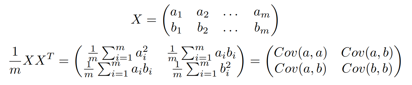
The diagonal elements of this matrix are the variances of the two variables, while the other elements are the covariances of a and b. The two are unified into a matrix. Similarly, if we have more than two features, the conclusion still holds.

Matrix diagonalization

We need to set all elements except those on the diagonal to 0, and arrange the elements on the diagonal by size from top to bottom. Assume that the covariance matrix corresponding to the original data matrix X is C, and assume that Y = PX. Let the covariance matrix of Y be D, let us deduce the relationship between D and C:

Therefore, our goal is finding a matrix P so that D is a diagonal matrix, and the elements located on the diagonal are arranged in order from large to small. The first K rows of P are the basis vectors to be found. Multiplying the matrix composed of the first K rows of P by X will reduce X from N dimensions to K dimensions and satisfy the above optimization conditions. We know that C is a real symmetric matrix, and for (n,n) real matrix, we can find n unit orthogonal eigenvectors E = e1, e2, … , en. Therefore, we have:

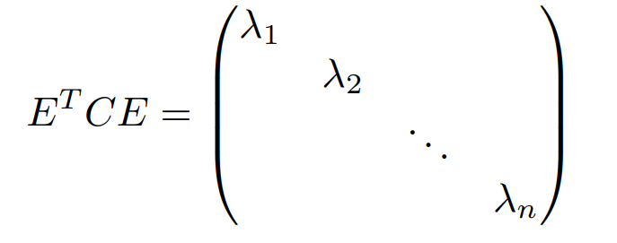
The elements on its diagonal are the eigenvalues corresponding to each eigenvector. Till now, we have found the matrix P, which is the transpose matrix of E.

Steps of PCA algorithm

Assume the shape of the original data is (n, m):

1. define a matrix X of the original data which shape is (n, m).
2. Subtract the mean of each feature and scale all the feature using mean-subtraction.
3. Calculate the covariance matrix C of X.
4. Find the eigenvalues and corresponding eigenvectors of C.
5. Arrange the eigenvectors into a matrix by rows from top to bottom according to the size of the corresponding eigenvalues, and take the first k rows to form the matrix P.
6. Matrix Y = PX is the data after dimensionality reduction to k dimensions.

Reconstruction from compressed representation

To reconstruction X from Y, we can use the following equation:

The reconstructed X_approx is the approximations of our original data, simply because we lost some information in dimensionality reduction.

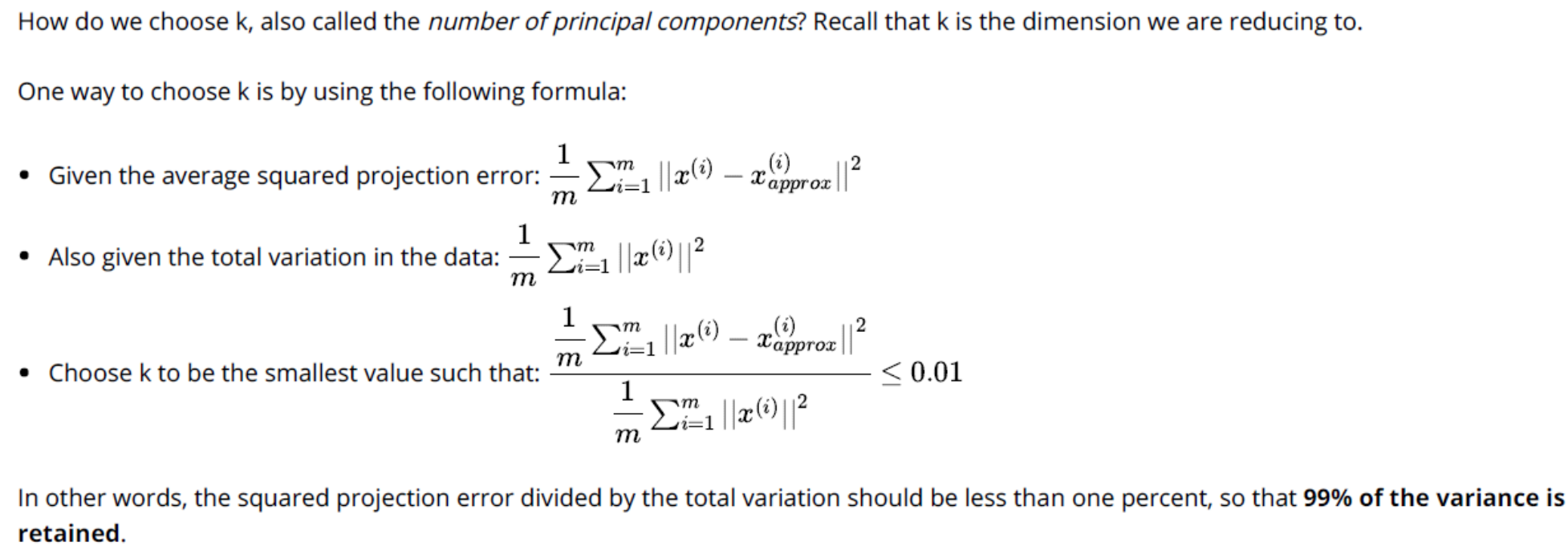
How to choose value of k (the dimension we are reducing to)

Suggestions when using PCA reduction

1. We should use PCA reduction only on the training set and not on the cross-validation or test sets. Instead, apply mapping to your cross-validation or test sets.
2. Trying to prevent overfitting. PCA may work when dealing with overfitting, but it is not recommended. Using just regularization will be at least as effective.
3. Do not assume you need to do PCA cause PCA will abandon part of information in your data set. Try your full machine learning algorithms firstly, and do PCA if you find that you truly need it.